Statement of the problem
In this post, we explain how to treat holes in a simple gated quantum dot simulation using the device from the Practical Application of the QTCAD Documentation. We use almost exactly the same code as in the Practical Application example #2, except that we modify applied potentials and doping, and configure the device to treat holes as quantum-confined charge carriers.
Special thanks to Kazuma Haruna from Osaka University for asking us about this topic.
Setting up the file structure
To run this example, copy-paste the contents of the qtcad/examples/practical_application directory in a separate folder. Keep only the first Python script (1-devicegen.py), which will be used to generate the 3D structure from the layout.
Then copy-paste the full code at the end of this post into a file called 2-poisson_schrodinger_holes.py. The simulation can then be run with
python qtcad/examples/practical_application/1-devicegen.py
python qtcad/examples/practical_application/2-poisson_schrodinger_holes.py
The rest of this post comments on specific code blocks of the Python script.
Discussion of the code
Importing libraries and setting up paths
## Import relevant libraries
from device import constants as ct
from device.mesh3d import Mesh, SubMesh
from device import io
from device import materials as mt
from device import analysis as an
from device import Device, SubDevice
from device.poisson import Solver as PoissonSolver
from device.poisson import SolverParams as PoissonSolverParams
from device.schrodinger import Solver as SchrodingerSolver
from device.schrodinger import SolverParams as SchrodingerSolverParams
import pathlib
import numpy as np

## Input files
script_dir = pathlib.Path(__file__).parent.resolve()
path_mesh = str(script_dir/'meshes'/'gated_dot.msh2')
Setting up the device
We first load the mesh and instantiate the device with
## Import and plot the mesh
scaling = 1e-6
mesh = Mesh(scaling,path_mesh)

## Create the device
# Use the 'conf_carriers' kwarg of the device to specify that holes will be the confined carrier
d = Device(mesh, conf_carriers='h')
d.set_temperature(0.1)

# Specify that the kp model to be used to describe holes will be the Luttinger-Kohn-Foreman model (4 bands)
d.hole_kp_model = "luttinger_kohn_foreman"
Compared with the previous case in which electrons were considered, the device constructor has an additionaly keyword argument (conf_carriers) which we set to 'h' for holes (it would be 'e' for electrons). In the last line, we also specify the kp model to be used to describe holes in the effective Schrödinger equation. Here, we use the Luttinger-Kohn-Foreman model. Though a 6-band model is also available with "luttinger_kohn_foreman_6band", here we use the default 4-band Luttinger-Kohn-Foremand model in which only the heavy-hole and light-hole bands are considered.
We then set up the regions and boundaries of the device, exactly as before, except for the doping type (positive doping instead of negative) and gate potential values.
## Set up device materials and boundaries
# Ionized dopant density
doping = 2e18*1e6   # In SI units

# Set up regions
d.new_region("cap", mt.GaAs)
d.new_region("barrier", mt.AlGaAs)
d.new_region("dopant_layer", mt.AlGaAs,pdoping=doping)
d.new_region("spacer_layer", mt.AlGaAs)
d.new_region("spacer_dot", mt.AlGaAs)
d.new_region("two_deg", mt.GaAs)
d.new_region("two_deg_dot", mt.GaAs)
d.new_region("substrate", mt.GaAs)
d.new_region("substrate_dot", mt.GaAs)

# Align the bands across hetero-interfaces using GaAs as the reference material
d.align_bands(mt.GaAs)

# Applied potentials
Vtop_1 = 0.
Vtop_2 = 0.
Vtop_3 = 0.
Vbottom_1 = 0.
Vbottom_2 = 0.
Vbottom_3 = 0.

# Work function of the metallic gates at midgap of GaAs
barrier = 0.834*ct.e    # n-type Schottky barrier height

# Set up boundary conditions
d.new_schottky_bnd("top_gate_1", Vtop_1, barrier)
d.new_schottky_bnd("top_gate_2", Vtop_2, barrier)
d.new_schottky_bnd("top_gate_3", Vtop_3, barrier)
d.new_schottky_bnd("bottom_gate_1", Vbottom_1, barrier)
d.new_schottky_bnd("bottom_gate_2", Vbottom_2, barrier)
d.new_schottky_bnd("bottom_gate_3", Vbottom_3, barrier)
d.new_ohmic_bnd("ohmic_bnd")
In addition, as in this forum post, we set the cap region to be a perfect insulator to suppress unwanted classical charges induced by Schottky gates.
# Make the cap an ideal insulator to suppress unphysical charges
d.new_insulator("cap")
Solving non-linear Poisson
We set up the dot region and non-linear Poisson solver exactly as before, and run it with
## Set up and run the solvers

# Create the non-linear Poisson solver and set its parameters
solver_params = PoissonSolverParams({"tol": 1e-3, "maxiter": 100})
poisson_solver = PoissonSolver(d, solver_params=solver_params)

# Create a submesh including only the dot region
submesh = SubMesh(mesh, ["spacer_dot","two_deg_dot","substrate_dot"])

# Set up the dot region in which no classical charge is allowed
d.set_dot_region(submesh)

# Solve Poisson
poisson_solver.solve()
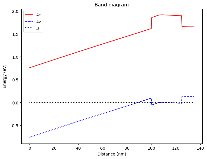
We may then plot a linecut of the band diagram along the z axis, exactly in the middle of the simulation domain in the xOy plane.
# Plot line cut of the bands right in the middle of the dot region
x, y, z = mesh.glob_nodes.T
xmin = np.min(x); xmax = np.max(x)
ymin = np.min(y); ymax = np.max(y)
zmin = np.min(z); zmax = np.max(z)
Lx = xmax-xmin; xc = (xmin+xmax)/2.
Ly = ymax-ymin; yc = (ymin+ymax)/2.
Lz = zmax-zmin; zc = (zmin+zmax)/2.
an.plot_bands(d,(xc,yc,zmin),(xc,yc,zmax))

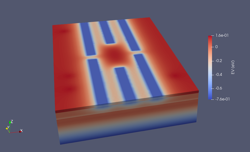
Finally, we can save the valence band edge in 3D in .vtu format.
# Save the valence band edge in .vtu format
outfile_vlnce_band_edge = str(script_dir / "output" / "vlnce_band_edge.vtu")
out_dict = {"EV (eV)": d.vlnce_band_edge()/ct.e}
io.save(outfile_vlnce_band_edge, out_dict, mesh)
The resulting file may be visualized in ParaView. The result is very similar to the conduction band edge for the previous simulations for electrons, except that now we expect holes to be confined near valence band edge maxima (instead of conduction band edge minima).

Solving Schrödinger
We set up and solve the Schrödinger solver exactly as before.
## Calculate the energy levels and envelope functions
# Get the potential energy from the band edge for usage in the Schrodinger solver
d.set_V_from_phi()

# Create a subdevice for the dot region
subdevice = SubDevice(d,submesh)

# Create a Schrodinger solver and solve
print("Solving effective Schrodinger's equation for holes")
schrod_solver = SchrodingerSolver(subdevice)
schrod_solver.solve()
We then print the eigenenergies with
# Print energies
subdevice.print_energies()
The result is
Energy levels (eV)
[0.05448565 0.05448557 0.05296507 0.05296485 0.05157031 0.05156969
 0.05124366 0.05124318 0.04984557 0.04984367]
We see that in the absence of an external magnetic field, the energy levels are split into nearly-exactly degenerate doublets (a difference between levels of order 10-100 neV persists because of the finite numerical precision of the Schrödinger solver, which may be improved if needed). These doublets correspond to heavy-hole and light-hole bands. In addition, heavy-hole and light-hole bands are split due to confinement within the quantum dot.
We may also visualize the hole envelope functions by saving them in .vtu format and plotting them in ParaView. We export the envelope functions with:
# Save the first few eigenstates
outfile_eigenfunctions = str(script_dir / "output" / "eigenfunctions.vtu")
out_dict = {"Ground, heavy-hole up, real": np.real(subdevice.eigenfunctions[:,0,0]),
    "Ground, heavy-hole down, real": np.real(subdevice.eigenfunctions[:,0,1]),
    "Ground light-hole up, real": np.real(subdevice.eigenfunctions[:,0,2]),
    "Ground light-hole down, real": np.real(subdevice.eigenfunctions[:,0,3]),
    "Ground, heavy-hole up, imag": np.imag(subdevice.eigenfunctions[:,0,0]),
    "Ground, heavy-hole down, imag": np.imag(subdevice.eigenfunctions[:,0,1]),
    "Ground light-hole up, imag": np.imag(subdevice.eigenfunctions[:,0,2]),
    "Ground light-hole down, imag": np.imag(subdevice.eigenfunctions[:,0,3])}
io.save(outfile_eigenfunctions, out_dict, submesh)
The eigenfunctions attribute of the subdevice object is a 3D array whose first index corresponds to global nodes of the mesh, whose second index labels the orbital quantum number, and whose third index labels bands (0 for heavy-hole up, 1 for heavy-hole down, 2 for light-hole up, and 3 for light-hole down). In addition, hole envelope functions are in general complex quantities, so that we save their real and imaginary parts separately. This means that 8 quantities must be exported to visualize all the components of the hole orbital ground state.
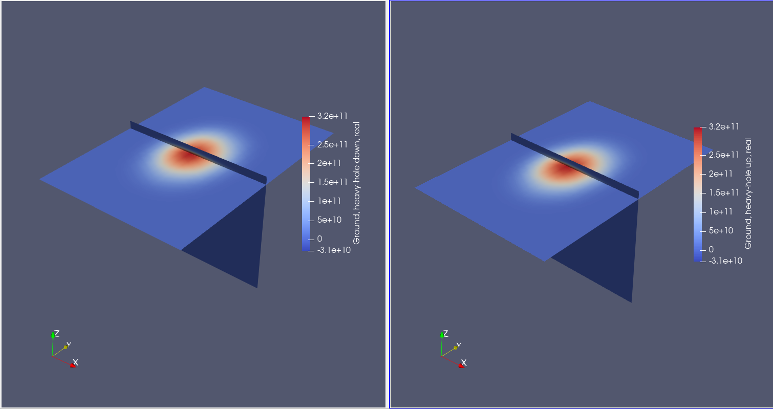
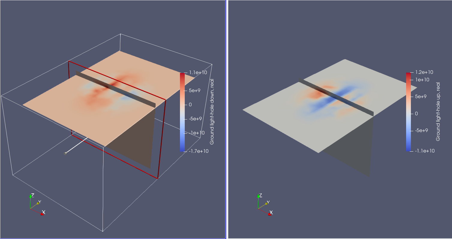
By plotting these quantities into ParaView, we quickly realize that the dominant contributions of the hole orbital ground state come from the heavy-hole up and heavy-hole down envelopes, and that these quantities are mostly real. Since no magnetic field is applied, arbitrary linear combinations of heavy-hole up and heavy-hole down states are equivalent -- however, this can be changed by applying a magnetic field and including the Zeeman effect, as in this tutorial.
Heavy hole envelope functions

Light hole envelope functions

Full code
## Import relevant libraries
from device import constants as ct
from device.mesh3d import Mesh, SubMesh
from device import io
from device import materials as mt
from device import analysis as an
from device import Device, SubDevice
from device.solver_params import SolverParams
from device.poisson import Solver as PoissonSolver
from device.schrodinger import Solver as SchrodingerSolver
import pathlib
import numpy as np

## Input files
script_dir = pathlib.Path(__file__).parent.resolve()
path_mesh = str(script_dir/'meshes'/'gated_dot.msh2')

## Import and plot the mesh
scaling = 1e-6
mesh = Mesh(scaling,path_mesh)

## Create the device
# Use the 'conf_carriers' kwarg of the device to specify that holes will be the confined carrier
d = Device(mesh, conf_carriers='h')
d.set_temperature(0.1)

# Specify that the kp model to be used to describe holes will be the Luttinger-Kohn-Foreman model (4 bands)
d.hole_kp_model = "luttinger_kohn_foreman"

## Set up device materials and boundaries
# Ionized dopant density
doping = 2e18*1e6   # In SI units

# Set up regions
d.new_region("cap", mt.GaAs)
d.new_region("barrier", mt.AlGaAs)
d.new_region("dopant_layer", mt.AlGaAs,pdoping=doping)
d.new_region("spacer_layer", mt.AlGaAs)
d.new_region("spacer_dot", mt.AlGaAs)
d.new_region("two_deg", mt.GaAs)
d.new_region("two_deg_dot", mt.GaAs)
d.new_region("substrate", mt.GaAs)
d.new_region("substrate_dot", mt.GaAs)

# Align the bands across hetero-interfaces using GaAs as the reference material
d.align_bands(mt.GaAs)

# Applied potentials
Vtop_1 = 0.
Vtop_2 = 0.
Vtop_3 = 0.
Vbottom_1 = 0.
Vbottom_2 = 0.
Vbottom_3 = 0.

# Work function of the metallic gates at midgap of GaAs
barrier = 0.834*ct.e    # n-type Schottky barrier height

# Set up boundary conditions
d.new_schottky_bnd("top_gate_1", Vtop_1, barrier)
d.new_schottky_bnd("top_gate_2", Vtop_2, barrier)
d.new_schottky_bnd("top_gate_3", Vtop_3, barrier)
d.new_schottky_bnd("bottom_gate_1", Vbottom_1, barrier)
d.new_schottky_bnd("bottom_gate_2", Vbottom_2, barrier)
d.new_schottky_bnd("bottom_gate_3", Vbottom_3, barrier)
d.new_ohmic_bnd("ohmic_bnd")

# Make the cap an ideal insulator to suppress unphysical charges
d.new_insulator("cap")

## Set up and run the solvers

# Create the non-linear Poisson solver and set its parameters
solver_params = SolverParams({"tol": 1e-3, "maxiter": 100}, problem="poisson")
poisson_solver = PoissonSolver(d, solver_params=solver_params)

# Create a submesh including only the dot region
submesh = SubMesh(mesh, ["spacer_dot","two_deg_dot","substrate_dot"])

# Set up the dot region in which no classical charge is allowed
d.set_dot_region(submesh)

# Solve Poisson
poisson_solver.solve()

# Plot line cut of the bands right in the middle of the dot region
x, y, z = mesh.glob_nodes.T
xmin = np.min(x); xmax = np.max(x)
ymin = np.min(y); ymax = np.max(y)
zmin = np.min(z); zmax = np.max(z)
Lx = xmax-xmin; xc = (xmin+xmax)/2.
Ly = ymax-ymin; yc = (ymin+ymax)/2.
Lz = zmax-zmin; zc = (zmin+zmax)/2.
an.plot_bands(d,(xc,yc,zmin),(xc,yc,zmax))

# Save the valence band edge in .vtu format
outfile_vlnce_band_edge = str(script_dir / "output" / "vlnce_band_edge.vtu")
out_dict = {"EV (eV)": d.vlnce_band_edge()/ct.e}
io.save(outfile_vlnce_band_edge, out_dict, mesh)

## Calculate the energy levels and envelope functions
# Get the potential energy from the band edge for usage in the Schrodinger solver
d.set_V_from_phi()

# Create a subdevice for the dot region
subdevice = SubDevice(d,submesh)

# Create a Schrodinger solver and solve
print("Solving effective Schrodinger's equation for holes")
schrod_solver = SchrodingerSolver(subdevice)
schrod_solver.solve()

# Print energies
subdevice.print_energies()

# Save the first few eigenstates
outfile_eigenfunctions = str(script_dir / "output" / "eigenfunctions.vtu")
out_dict = {"Ground, heavy-hole up, real": np.real(subdevice.eigenfunctions[:,0,0]),
    "Ground, heavy-hole down, real": np.real(subdevice.eigenfunctions[:,0,1]),
    "Ground light-hole up, real": np.real(subdevice.eigenfunctions[:,0,2]),
    "Ground light-hole down, real": np.real(subdevice.eigenfunctions[:,0,3]),
    "Ground, heavy-hole up, imag": np.imag(subdevice.eigenfunctions[:,0,0]),
    "Ground, heavy-hole down, imag": np.imag(subdevice.eigenfunctions[:,0,1]),
    "Ground light-hole up, imag": np.imag(subdevice.eigenfunctions[:,0,2]),
    "Ground light-hole down, imag": np.imag(subdevice.eigenfunctions[:,0,3])}
io.save(outfile_eigenfunctions, out_dict, submesh)