Statement of the problem
In most if not all gated quantum dot geometries, electrons or holes are confined in a given host semiconductor (such as silicon or gallium arsenide), while a semiconductor with a wider bandgap or an oxide is used to create a potential barrier that separates confined carries from electrostatic gates used to tune the potential wells. In such cases, applying a strong gate potential may result in a situation in which the conduction (valence) band edge goes below (above) the Fermi level near the interface with a gate. Unless otherwise specified, and if this region of space does not belong to the quantum-dot region, the non-linear Poisson solver will then assign a significant charge density near the gate interface. This may however not be physical, since at cryogenic temperature and for sufficiently wide potential barriers, it may be impossible for charge carriers to tunnel from the doped regions to this region near the interface.
In this post, we first illustrate this issue considering the gated quantum dot device from the Practical Application of the QTCAD Documentation. We use almost exactly the same code as in the Practical Application example #2, except that we modify some of the applied potentials. Next, we explain how to resolve the issue using a simple QTCAD command.
Illustration of the problem
We first produce the mesh by running
python qtcad/examples/practical_application/1-devicegen.py
The mesh is then saved into the qtcad/examples/practical_application/meshes directory.
The next step is to run Practical Application #2 with modified potentials. To do so, we replace the code block defining applied gate potentials by:
# Applied potentials
Vtop_1 = -1.0
Vtop_2 = -1.0
Vtop_3 = -1.0
Vbottom_1 = -1.0
Vbottom_2 = -1.0
Vbottom_3 = -1.0
In other words, we change the applied potential from -0.5 V to -1.0 V.
In addition, here we are only interested in the Poisson solver behavior. Therefore, instead of instantiating and running the Schrödinger solver, and outputting vtu files, we simply plot the band diagram and hole density below top gate 2 with
# Plot the band diagram along a vertical linecut right below the top 2 gate
x, y, z = d.mesh.glob_nodes.T
an.plot_bands(d, (235e-9,500e-9,np.max(z)), (235e-9,500e-9,np.min(z)))

# Plot the hole density along the same linecut
an.plot_linecut(mesh, d.p/1e6, (235e-9,500e-9,np.max(z)),
    (235e-9,500e-9,np.min(z)), title = "Hole density (cm$^{-3}$)")
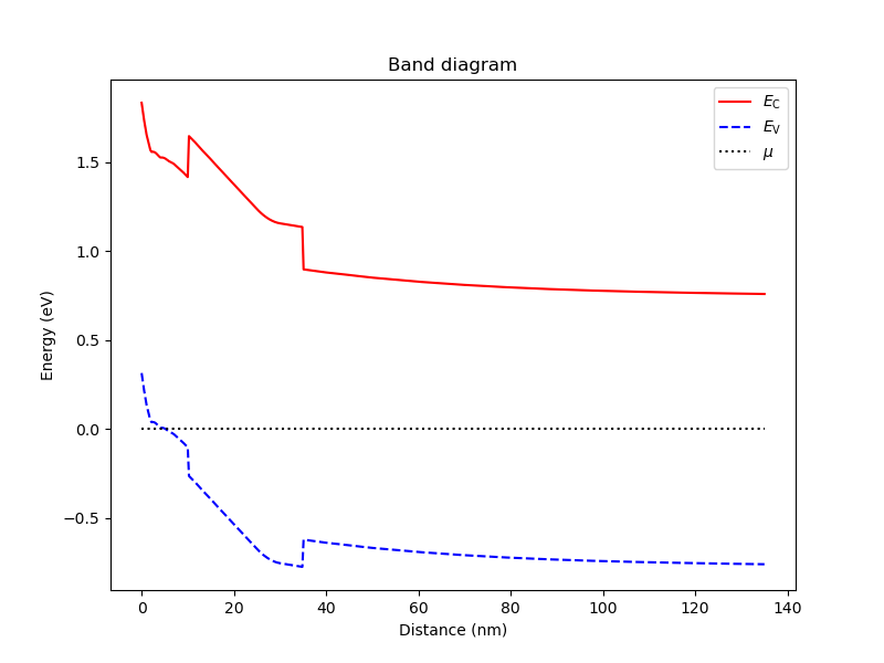
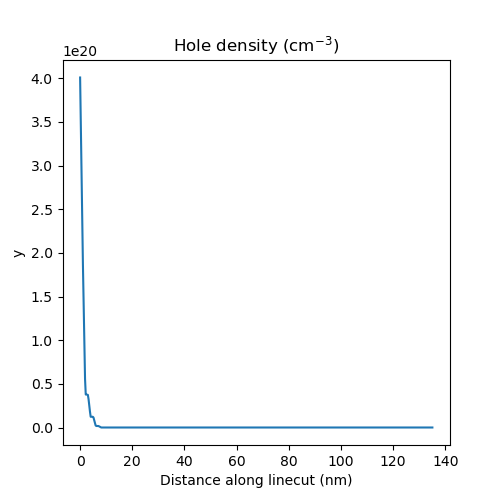
Running the code, we find that the error in the non-linear Poisson solver saturates to 0.02 V after 18 iterations. In other words, the solver fails to converge within the prescribed tolerance. To understand this, we look at the band diagram, and at the hole density.


We see that for such strongly negative potentials, the valence band edge is significantly above the Fermi level, which leads to strong accumulation of charge from holes. In addition to being potentially unphysical, such strong charge accumulation is detrimental to convergence of the non-linear Poisson solver.
Suppressing the unwanted charges
To suppress the unwanted charges, right after defining the regions of the device, we define the cap region as an ideal insulator with the command
# Set the cap to be an ideal insulator, in which:
## 1) The classical charge density is set to exactly zero
## 2) The carrier wave functions are forced to zero in the Schrödinger solver
d.new_insulator("cap")
In an ideal insulator:
- The classical charge density is set to exactly zero;
- The carrier wave functions are forced to zero in the Schrödinger solver.
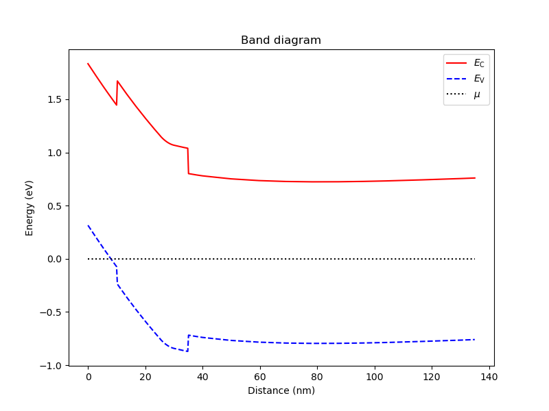
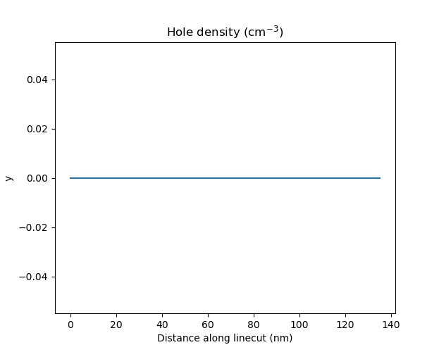
In the present case, this enables the non-linear Poisson solver to converge. In addition, plotting the band diagram, we see that no band bending is visible in the region near the top gate 2, implying that no charges accumulate there. This is confirmed by plotting the hole density along the same linecut.


Acknowledgments
Special thanks to Prof. Takafumi Fujita from Osaka University for bringing up this important topic to our attention.
Full code
__copyright__ = "Copyright 2022, Nanoacademic Technologies Inc."

import pathlib
import numpy as np

from device import constants as ct
from device.mesh3d import Mesh, SubMesh
from device import materials as mt
from device import Device
from device.solver_params import SolverParams
from device.poisson import Solver as PoissonSolver
from device import analysis as an

# Input file
script_dir = pathlib.Path(__file__).parent.resolve()
path_mesh = str(script_dir/'meshes'/'gated_dot.msh2')

# Load the mesh
scaling = 1e-6
mesh = Mesh(scaling,path_mesh)

# Create device
d = Device(mesh)
d.set_temperature(0.1)

# Ionized dopant density
doping = 3e18*1e6   # In SI units

# Set up materials in heterostructure stack
d.new_region("cap", mt.GaAs)
d.new_region("barrier", mt.AlGaAs)
d.new_region("dopant_layer", mt.AlGaAs,ndoping=doping)
d.new_region("spacer_layer", mt.AlGaAs)
d.new_region("spacer_dot", mt.AlGaAs)
d.new_region("two_deg", mt.GaAs)
d.new_region("two_deg_dot", mt.GaAs)
d.new_region("substrate", mt.GaAs)
d.new_region("substrate_dot", mt.GaAs)

# Set the cap to be an ideal insulator, in which:
## 1) The classical charge density is set to exactly zero
## 2) The carrier wave functions are forced to zero in the Schrödinger solver
## Uncomment the next line of code to use the ideal insulator option
# d.new_insulator("cap")

# Align the bands across hetero-interfaces using GaAs as the reference material
d.align_bands(mt.GaAs)

# Applied potentials
Vtop_1 = -1.0
Vtop_2 = -1.0
Vtop_3 = -1.0
Vbottom_1 = -1.0
Vbottom_2 = -1.0
Vbottom_3 = -1.0

# Work function of the metallic gates at midgap of GaAs
barrier = 0.834*ct.e    # n-type Schottky barrier height

# Set up boundary conditions
d.new_schottky_bnd("top_gate_1", Vtop_1, barrier)
d.new_schottky_bnd("top_gate_2", Vtop_2, barrier)
d.new_schottky_bnd("top_gate_3", Vtop_3, barrier)
d.new_schottky_bnd("bottom_gate_1", Vbottom_1, barrier)
d.new_schottky_bnd("bottom_gate_2", Vbottom_2, barrier)
d.new_schottky_bnd("bottom_gate_3", Vbottom_3, barrier)
d.new_ohmic_bnd("ohmic_bnd")

# Create the non-linear Poisson solver and set its parameters
solver_params = SolverParams({"tol": 1e-3, "maxiter": 100}, problem="poisson")
# solver_params = SolverParams({"tol": 1e-3, "maxiter": 10}, problem="poisson")
poisson_solver = PoissonSolver(d, solver_params=solver_params)

# Create a submesh including only the dot region
submesh = SubMesh(mesh, ["spacer_dot","two_deg_dot","substrate_dot"])

# Set up the dot region in which no classical charge is allowed
d.set_dot_region(submesh)

# Solve
poisson_solver.solve()

# Plot the band diagram along a vertical linecut right below the top 2 gate
x, y, z = d.mesh.glob_nodes.T
an.plot_bands(d, (235e-9,500e-9,np.max(z)), (235e-9,500e-9,np.min(z)))

# Plot the hole density along the same linecut
an.plot_linecut(mesh, d.p/1e6, (235e-9,500e-9,np.max(z)),
    (235e-9,500e-9,np.min(z)), title = "Hole density (cm$^{-3}$)")